Mastering Motion: An Analysis Primer on Uniformly Accelerated Rectilinear Motion

1. Foundations of Rectilinear Motion

To describe the physical universe—from the circulation of blood in arteries to the grand revolution of the Earth around the Sun—we must first establish a framework for motion. In physics, motion is defined as a change in the position of an object over time. While real-world objects have complex shapes and internal movements, we begin our study with rectilinear motion, which is motion strictly along a straight line.

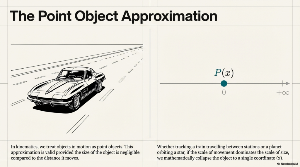
To simplify these complexities without sacrificing analytical rigor, we employ the point object approximation. This model allows us to treat a car, a train, or even a planet as a single point-like mass. This approximation is scientifically valid whenever the size of the object is significantly smaller than the distance it traverses. By adopting this simplification, we reduce the motion of a sprawling system to the motion of a single coordinate, making the underlying physics accessible.

Concept Spotlight: Motion Motion is the continuous change in the position of an object relative to a chosen frame of reference over time.

The “So What?” of Point Objects Treating a massive object as a point is the first step in “architecting” a physics problem. It allows us to neglect rotational and internal vibrations, focusing entirely on the object’s translational path. This simplification provides the necessary foundation for using algebraic and calculus-based tools to predict future states of motion with remarkable precision.

To accurately describe how an object’s position evolves, we must define the rates of change known as velocity and speed.

——————————————————————————–

2. Velocity vs. Speed: Measuring Change at an Instant

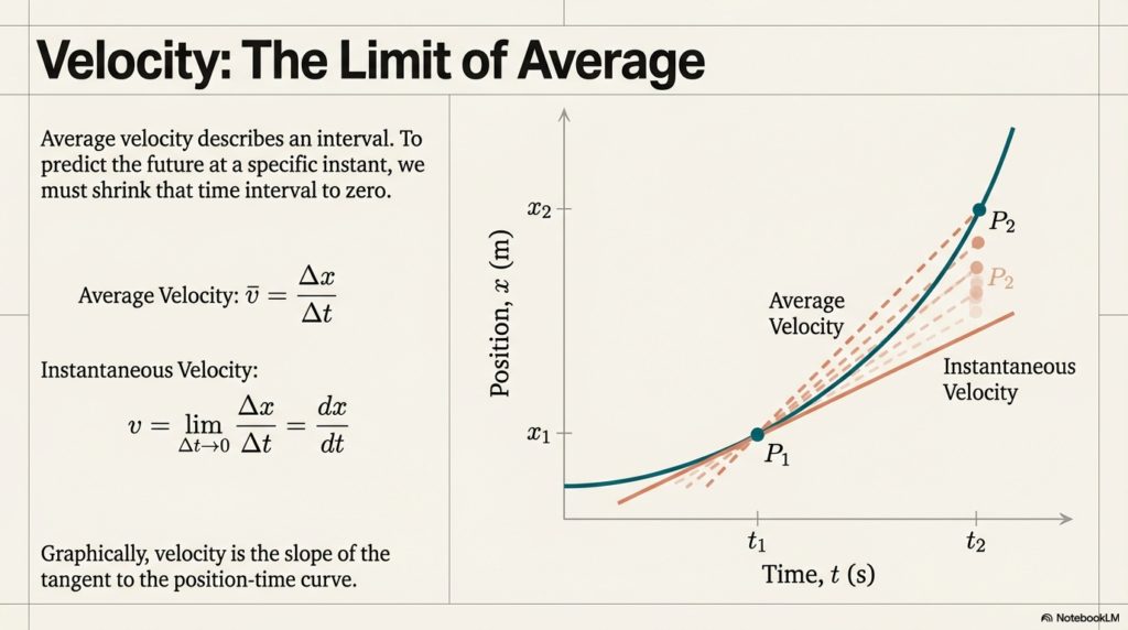
In formal kinematics, we must distinguish between an “overall” view of motion and the state of motion at a specific moment. The average velocity provides a broad summary over a finite time interval, but it fails to capture the nuances of a journey. For a truly precise analysis, we turn to the instantaneous velocity (v), which is the rate of change of position at a specific instant.

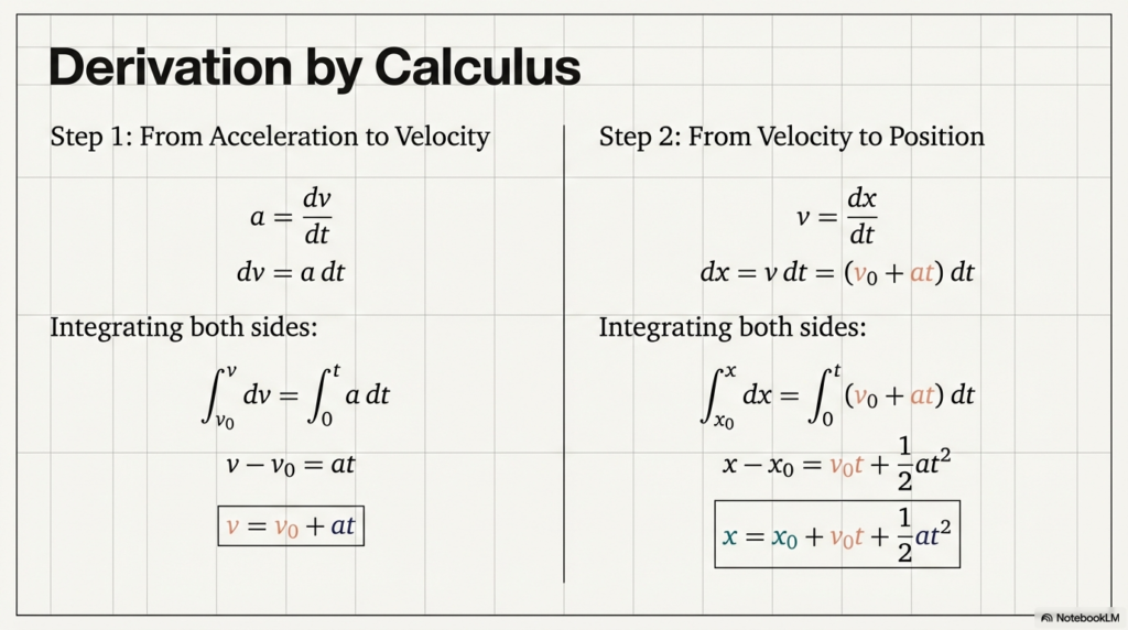
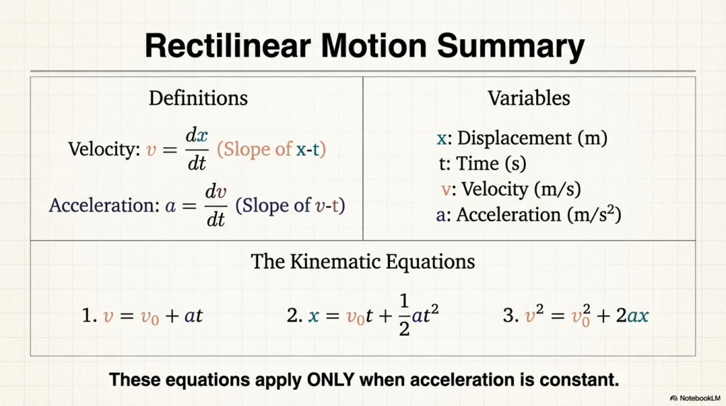
Mathematically, instantaneous velocity is the differential coefficient of position (x) with respect to time (t): v = \lim_{\Delta t \to 0} \frac{\Delta x}{\Delta t} = \frac{dx}{dt}

Feature	Average Velocity/Speed	Instantaneous Velocity/Speed
Time Interval	Measured over a finite interval (\Delta t).	Measured over an infinitesimally small interval (\Delta t \to 0).
Mathematical Representation	\Delta x / \Delta t	The derivative \frac{dx}{dt}
Physical Context	The displacement-to-time ratio for a trip.	The “speedometer” reading with a direction at any given t.

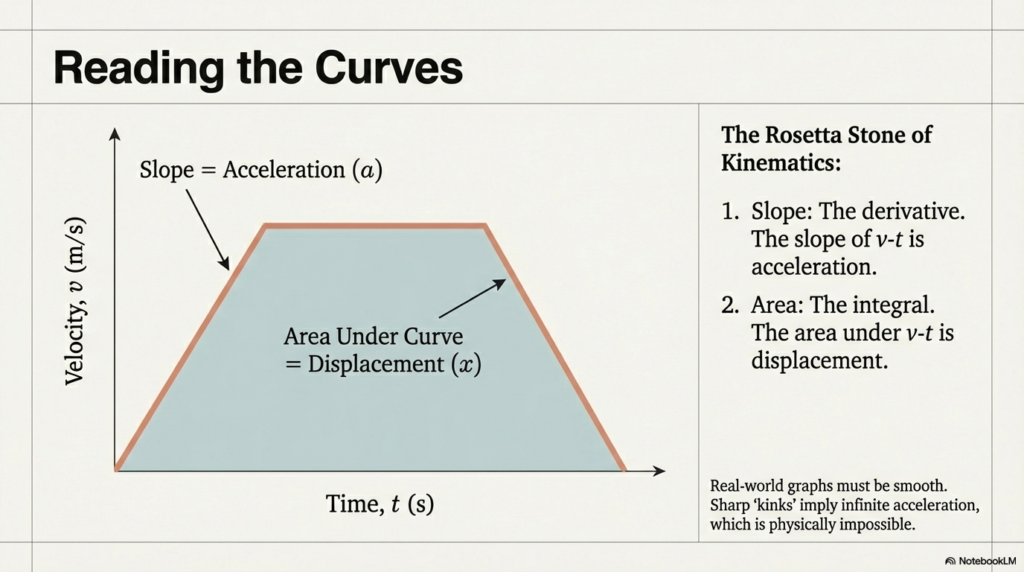
Graphical Insight On a position-time (x-t) graph, the instantaneous velocity is equal to the slope of the tangent to the curve at that specific point. As the time interval \Delta t shrinks toward zero, the line connecting two points on the curve converges into this tangent line, representing the exact rate of change.

Understanding Instantaneous Speed

• Magnitude Equivalence: Instantaneous speed is always the magnitude of instantaneous velocity. While a car might have a velocity of -25\text{ m/s} (moving in the negative direction), its speed is simply 25\text{ m/s}.
• Direction Independence: Speed is a scalar quantity; it does not account for the direction of travel.
• Consistency at the Limit: Unlike average speed (which can be greater than the magnitude of average velocity), at an infinitesimally small instant, the path length is identical to the magnitude of displacement.

When velocity itself changes over time, we introduce the dynamic concept of acceleration.

——————————————————————————–

3. Acceleration: The Dynamics of Changing Velocity

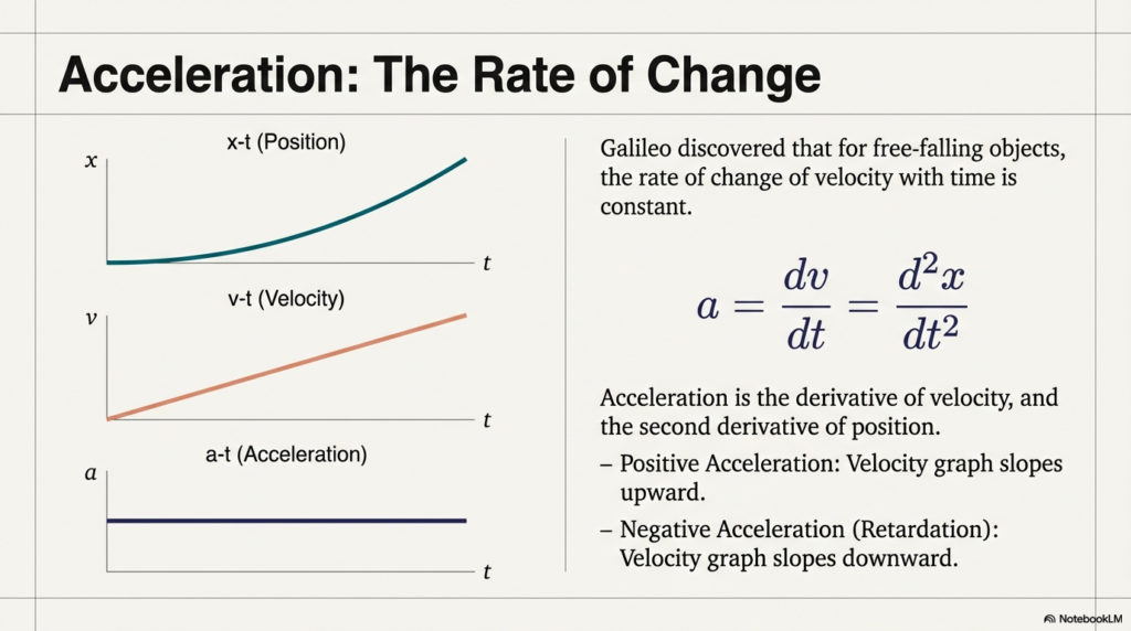
Acceleration (a) is the rate at which an object’s velocity changes with time. In the language of calculus, it is the derivative of velocity: a = \frac{dv}{dt}

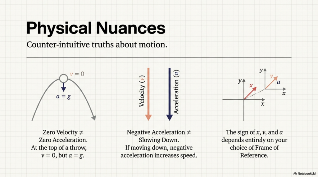
The Importance of the Coordinate System Before assigning a sign (+ or -) to acceleration, a learner must define their coordinate system. Signs are not absolute; they are relative to the chosen origin and axis. If we define “up” as positive, the acceleration due to gravity is negative. If we define “down” as positive, that same gravity becomes positive.

Categorizing Acceleration

• Positive Acceleration: Acceleration acts in the same direction as the chosen positive axis.
• Negative Acceleration: Acceleration acts in the direction opposite to the positive axis. Note: If an object is moving in the negative direction, a negative acceleration will cause it to speed up (speeding up occurs when velocity and acceleration share the same sign).
• Zero Acceleration (Uniform Motion): Velocity remains constant. The x-t graph is a straight line, and the v-t graph is a horizontal line.

The “Zero Velocity” Paradox A critical insight for any physics student: zero velocity does not necessarily imply zero acceleration. Consider a ball thrown vertically upward. At the very peak of its flight, its velocity is momentarily zero. However, its acceleration remains 9.8\text{ m/s}^2 downward. If the acceleration were also zero at that point, the ball would simply hang in the air forever.

For the specific case where this acceleration is constant, we can apply the Three Pillars of Kinematics.

——————————————————————————–

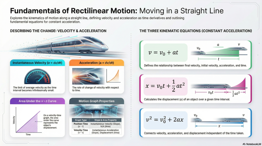
4. The Three Pillars: Kinematic Equations for Uniform Acceleration

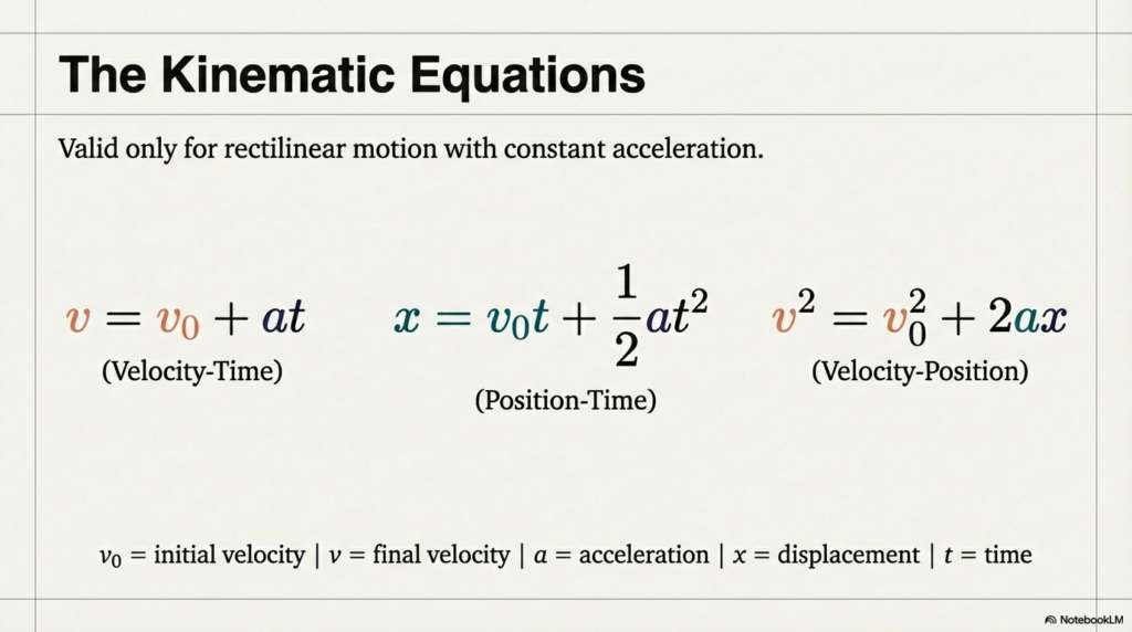
When acceleration is constant, the average acceleration equals the instantaneous acceleration. We can then derive three foundational equations that relate five variables: displacement (x), initial velocity (v_0), final velocity (v), acceleration (a), and time (t).

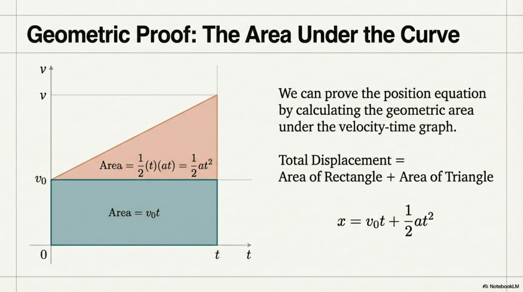
Graphical Derivation The displacement (x) of an object is represented by the area under the velocity-time (v-t) curve. For an object with constant acceleration, the area under the v-t line from t=0 to t forms a trapezoid. This area can be split into a rectangle (representing the initial velocity’s contribution: v_0 t) and a triangle (representing the displacement due to acceleration: \frac{1}{2}at^2). Summing these yields our second kinematic equation.

Kinematic Cheat Sheet

Equation	Variables Involved	Variable Missing	Primary Use Case
v = v_0 + at	v, v_0, a, t	x	To find final velocity when displacement is unknown.
x = v_0 t + \frac{1}{2}at^2	x, v_0, t, a	v	To find displacement when final velocity is unknown.
v^2 = v_0^2 + 2ax	v, v_0, a, x	t	To find velocity or displacement when time is unknown.

Note: In these equations, the displacement x is often the arithmetic average of the initial and final velocities multiplied by time: x = \left(\frac{v + v_0}{2}\right)t. If the object starts at a non-zero origin, substitute x with (x – x_0).

These abstract tools allow us to solve real-world problems involving gravity and automotive safety.

——————————————————————————–

5. Real-World Applications: Free Fall and Safety

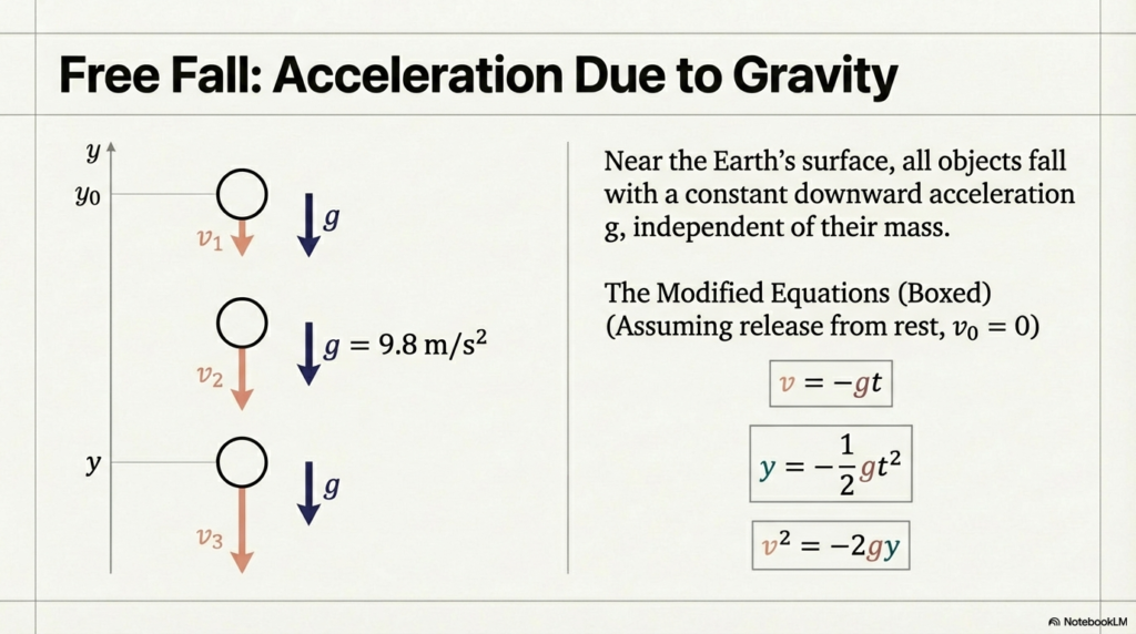
Uniformly accelerated motion is most commonly observed in Free Fall. Near the Earth’s surface, all objects (neglecting air resistance) fall with a constant acceleration due to gravity (g \approx 9.8\text{ m/s}^2).

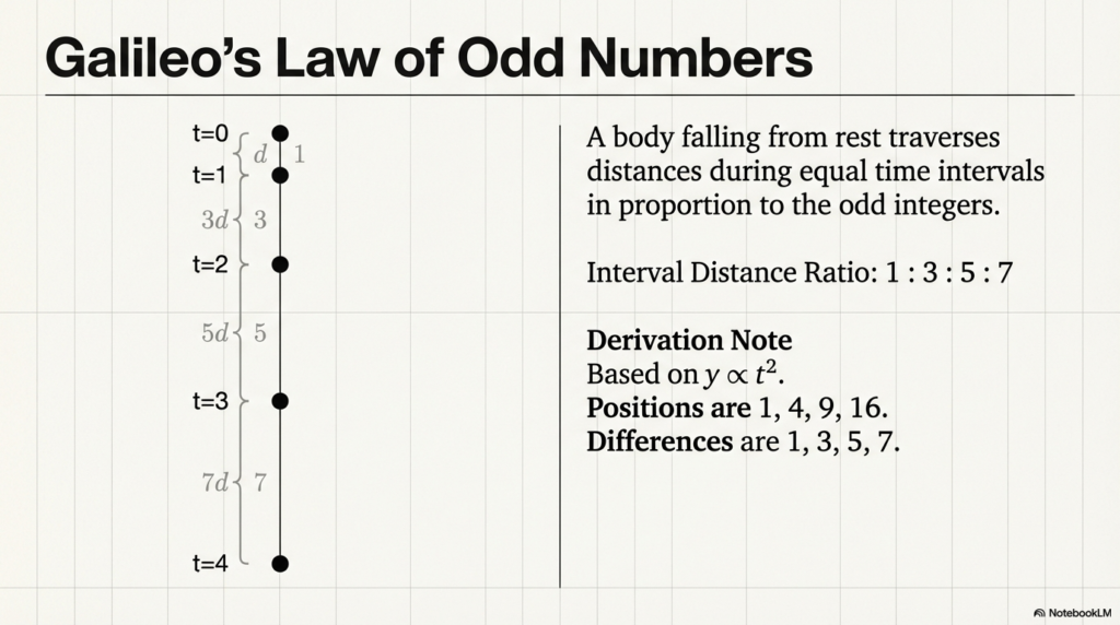
Galileo’s Law of Odd Numbers

Galileo proved that for any object falling starting from rest (v_0 = 0), the distances traversed in successive equal intervals of time follow a specific ratio.

1. Divide the time of fall into equal intervals \tau.
2. Calculate the position at t = \tau, 2\tau, 3\tau, \dots
3. The distances traveled in each successive interval follow the ratio of 1 : 3 : 5 : 7 : 9… This law confirms that the distance fallen is proportional to the square of the time elapsed.

Practical Insight: Stopping Distance

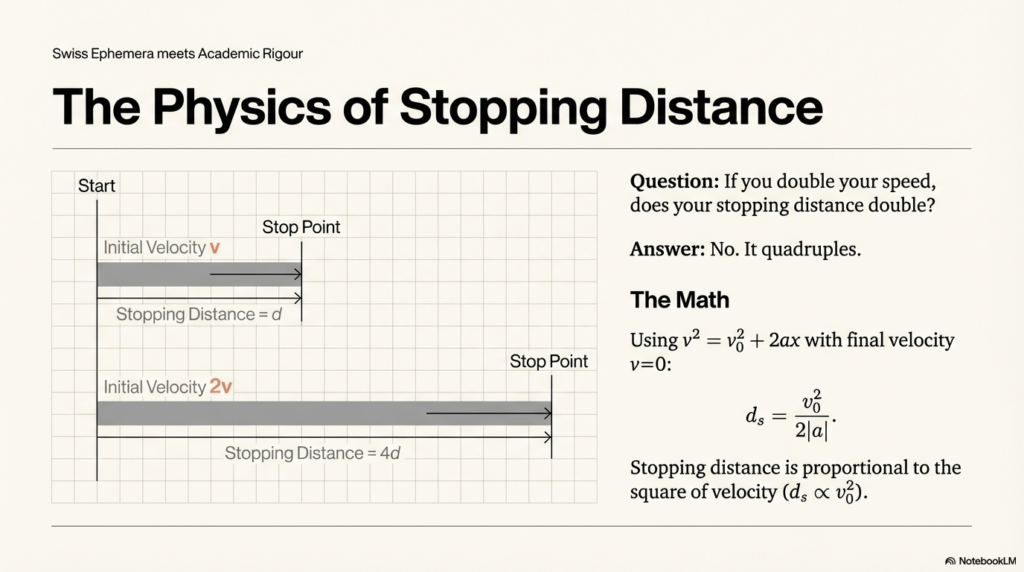
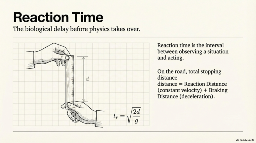
The kinematic equations are essential for determining the stopping distance (d_s)—the distance a vehicle travels after brakes are applied before coming to a complete rest.

Safety Note: The Stopping Formula Based on the equation v^2 = v_0^2 + 2ax, with a final velocity v = 0, the stopping distance is: d_s = \frac{-v_0^2}{2a} The “So What?”: Because the initial velocity (v_0) is squared, the stopping distance is proportional to the square of the speed. Doubling your initial velocity quadruples your stopping distance. This non-linear relationship is the primary reason why even small increases in speed significantly impact road safety.

By mastering these equations and conceptual nuances, we can precisely predict the trajectory and state of any object in uniform motion, providing a deterministic view of the physical world.

Object or Scenario	Initial Velocity (u)	Final Velocity (v)	Acceleration (a)	Time Interval (t)	Displacement (x/y)	Motion Type	Source
Ball thrown vertically upwards (Ex 2.3a, 2.3b, 2.6 Exercise)	20 m s−1 or 29.4 m s−1	0 m s−1 (at peak)	−10 m s−2 or −9.8 m s−2	2 s to 5 s	20 m (peak) or −25 m (relative to launch)	Free fall	[1]
Object in free fall (general case)	0 m s−1	−9.8t m s−1	−9.8 m s−2	t	−4.9t2 m	Free fall	[1]
Ball dropped from height (Ex 2.8 Exercise)	0 m s−1	Not in source	9.8 m s−2	12 s	90 m	Free fall with collisions	[1]
Ruler dropped for reaction time (Ex 2.7)	0 m s−1	Not in source	−9.8 m s−2	≈0.2 s	21.0 cm	Free fall	[1]
Object moving along x-axis (Ex 2.1)	0 m s−1 (at t=0 s)	10 m s−1 (at t=2.0 s)	5.0 m s−2	2.0 s	30 m (between 2 s and 4 s)	Constant acceleration	[1]
Car braking on highway (Ex 2.5 Exercise)	126 km h−1	0 km h−1	Not in source	Not in source	200 m	Constant acceleration	[1]
Woman walking to office (Ex 2.3 Exercise)	5 km h−1	5 km h−1	0 m s−2	0.5 h	2.5 km	Uniform motion	[1]
Woman returning from office (Ex 2.3 Exercise)	25 km h−1	25 km h−1	0 m s−2	0.1 h	2.5 km	Uniform motion	[1]
Motion of a car (numerical method)	Not in source	3.84 m s−1	Not in source	4 s	x=0.08t3	Non-uniform acceleration	[1]